ANALYSIS-CORRELATION-FUNCTIONS
| Field | Value |
|---|---|
| Name | [Analysis] Correlation Functions |
| Slug | 188 |
| Status | raw |
| Category | Informational |
| Editor | Alexander Mozeika [email protected] |
| Contributors | Filip Dimitrijevic [email protected] |
Timeline
- 2026-05-29 —
67e498e— chore: fix math issues (#350) - 2026-05-28 —
d45eed2— Chore: mirror blochain specs into github/mdbook (#347)
Revision History
| Version | Changes | Date |
|---|---|---|
| 1.0.0 | Initial revision. | 2025-09-08 |
Introduction
One of possible approaches to design a reliable anonymous communication (AC) system is to reduce statistical correlations between communicating nodes. Here we model a network of communicating nodes as a probabilistic discrete-state cellular automata (CA). We consider a node-centred approach where a node has associated with it variable representing its discrete state, such as sending, receiving, etc. Also we suggest a more granular connection-centred approach where discrete states of communication links of a node are considered. We note that message-centred approach is also possible but not pursued here. Finally, we discuss functions which can be used to quantify correlations in empirical analysis of AC systems.
The “cellular automata” (CA) model
- The system we consider is a network of communicating nodes where nodes are labelled by the set .
- We assume that nodes receive and send messages and these messages are indistinguishable, i.e. it is either impossible to observe bitstreams of messages, or incoming and outgoing messages are bitwise uncorrelated.
- The node at time can be in the state of either sending (message) or receiving (message) or inactive, i.e. neither sending or receiving. The latter is modelled by the variable as follows
| | Node at time is |
|---|---|
| -1 | sending a message |
| 0 | inactive |
| 1 | receiving a message |
- We note that a node can be in more states, for example in addition to sending, receiving, and inactive it could have an additional state of simultaneous sending and receiving, i.e. “send-receive” state. Additional states c can be modelled by extending the alphabet from which takes its values, i.e. for the most general case.
- The vector is the state of the network at time and for , where , the (ordered by time) set of vectors is the path, through the state-space , taken by the system from the time to the time . The latter can be represented by a table (or matrix) as in the example below obtained from simulations.
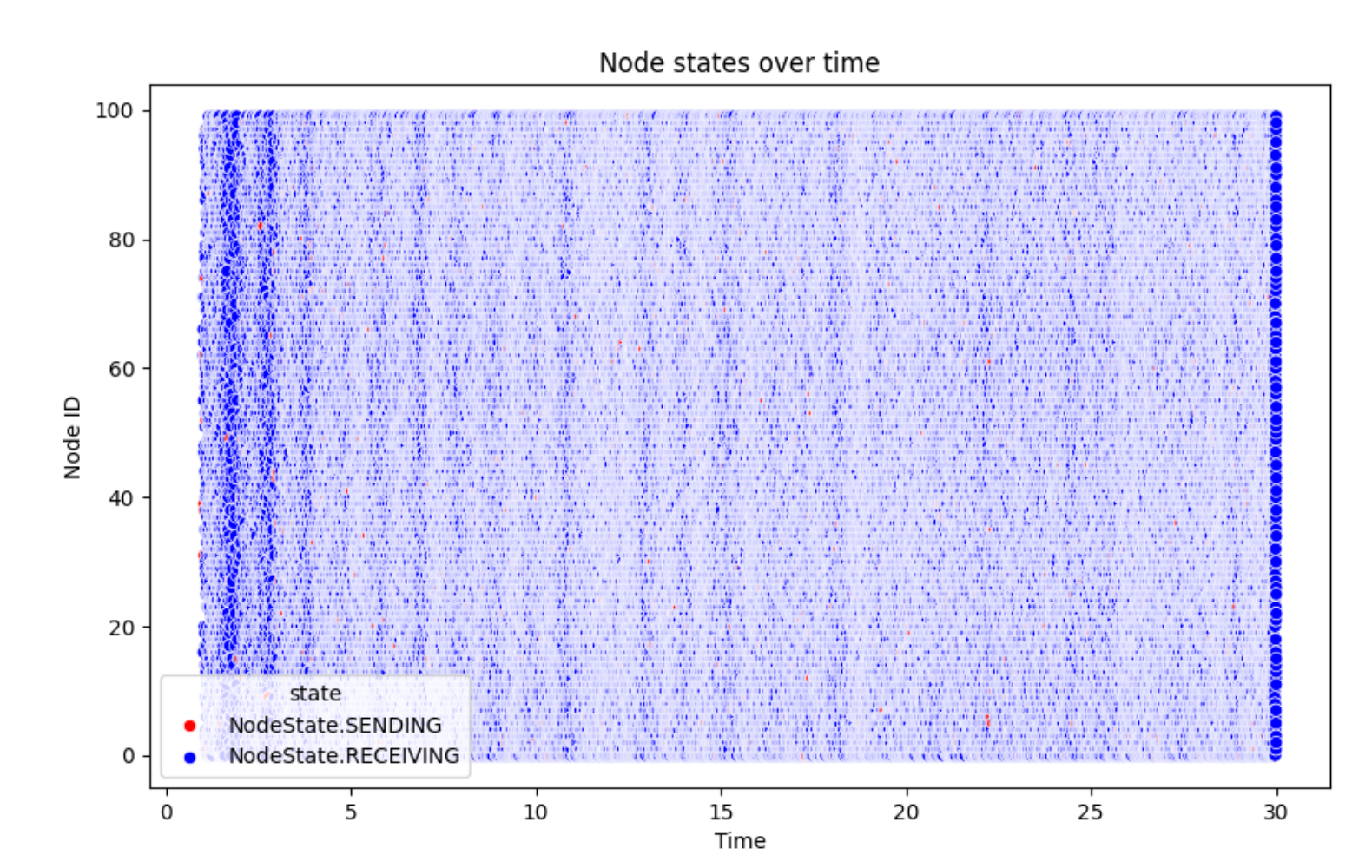
The state of the network as a function of time. The node at time , represented by dot, is either sending (red dot) or receiving (blue dots) or inactive (white dot). All nodes are sending messages through nodes with .
- Here we expect that dynamics of the network state is Markovian, i.e. depends only on , and can be described by the probability . We note if the latter is factorises, i.e. , for all then nodes are uncorrelated and “observing” any given node doesn’t reveal any information about the other node/nodes.
- To take this research route further would require to derive master equation for , to derive and analyse equations for correlation functions, etc.
Empirical analysis of correlations in CA model
- If node at time is in the state then the Kronecker delta function is defined as follows
- The sum counts how many times node i was in state on the (ordered) set of times , where . Additionally, the latter can be used to define the (empirical) frequency .
- The sum counts number of nodes in the network which are in state at time and can be used to define the (empirical) frequency .
- The sum counts how many nodes in the network were in state at time and in state at time , where , can be used to define the joint (empirical) frequency (or correlation function) .
- In a similar manner we can define the (spatial) correlation function
- In above the sum counts how many pairs of distinct nodes in the network (there are such pairs in total ) were in state and at, respectively, the time and
Node-centred approach
- We adopt the CA model where state of AC system at time is described by the vector , where the variable is the state of node , such as receiving a message, sending a message, etc., at time . For example , where corresponds to sending, corresponds to inactive and corresponds to receiving.
- We note that a node connected to more than two nodes can be receiving and/or sending multiple messages at the same time. However, to simplify analysis we will assume that at any time a node can receive (or send) at most one message.
- We assume that we have observed such vectors at times collected in the (ordered) set , where .
| | | | | | |
|---|---|---|---|---|---|
| | -1 | 0 | 1 | | -1 |
| | 0 | 1 | 0 | | 1 |
| | | | | | |
| | -1 | 0 | -1 | | 1 |
| | 1 | 0 | -1 | | 1 |
| | | | | | |
| | 0 | 0 | 0 | | 1 |
- We define the indicator function: when and otherwise, i.e. this is the Kronecker delta function. The latter allows us to define various “correlation functions” such as the (empirical) frequency , the joint frequency , etc.
- In general the product could be used to construct any correlation function.
Connection-centred approach
- The state of node , with respect to its connection to the node , at time is described by the variable , where corresponds to node sending message to node , corresponds to “no-communication” state between nodes and corresponds to node receiving a message from node .
- We could use an extended alphabet as additional states may exist. For example, it is possible that node is both simultaneously sending a message to node and receiving a message from , i.e. node is in “send-receive” state. This situation can be modelled by the variable , where corresponds to “no-communication” state between nodes, corresponds to node sending message to node , corresponds to node i in “send-receive” state and corresponds to node receiving a message from node .
- Let us define the set of nodes connected to the node as the (ordered) set ( notation here means “neighbourhood” of node ) then the state of node , with respect to all of its connections, at time is the (ordered by ) set (or vector) , i.e. the state of its connections at time . We note that “no-communication” and not being a member of are different concepts.
- Using above definition the state of all nodes at time can be described by the “vector”
- We note that , i.e. can be any ternary string of length . Hence can be represented by a single number from the set once the mapping between the sets and is fixed.
- For we can define the frequency for node as follows
where , which “counts” how many times connections of node , with respect to , were in some specific communication “pattern” .
- In a similar manner for and we can define the joint frequency
for nodes and .
Mutual information
- For the joint frequency the (empirical) mutual information can be used as a measure of dependence between states of node and . The latter can be used in both node-centric and connection-centric approaches.
Hamming distance
- The (normalised) Hamming distance between the vectors and is the sum , i.e. the number of disagreements between the and is counted and divided by .
- We note when is set (or vector) as in the section on connection-centric approach then , i.e. the latter is if and only if states of all connections of node in and are the same.
- We note that with when and 1 when for all .
- Assuming that we observe the states and of two systems on the same time-set , where , the (average) Hamming distance measures how these two systems are different. We note that with when for all and when for all and all .
- Let us assume we observed at times the states and of two copies of exactly the same AC system. That is the graph is the same in both copies, with exactly the same LEVEL 0 noise, i.e. if node in copy , described by , is sending a (LEVEL 0) message then node in copy , described by , is also sending the same message, etc. We note that the latter can be achieved in simulation which usually uses pseudo-randomness and hence evolution of AC system in time is deterministic. The latter implies that for all and hence in this case .
- Let us now, without loss of generality, assume that node in the copy , described by , sent a LEVEL 2 message, through the nodes , to the node at time and node received this message at time .
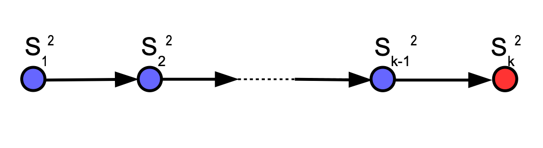
- We note that for we have because states of copies 1 and 2, described by and , are exactly the same before this event. For times we can have , i.e. the states of copies and , described by and , are different after the event at .